Message-Passing Graph Neural Networks from Scratch: GCN and GAT in Pure PyTorch
Abstract
Graph neural networks operate on observations whose geometry is specified by relations rather than by a regular grid. Their central computation is local: each node constructs messages from its neighbors, aggregates them without depending on neighbor order, and updates its representation. This article develops that computation from first principles and specializes it to two canonical architectures: the Graph Convolutional Network (GCN) and the Graph Attention Network (GAT).
The implementations use ordinary PyTorch tensors only. In particular, they do not use PyTorch Geometric, GCNConv, GATConv, or a message-passing base class. This is an educational choice: sparse edge indexing, neighborhood normalization, attention coefficients, and scatter aggregation remain explicit. The complete implementation and reproducible experiments are available in the companion repository.
1. Graph data
1.1 Definition and attributes
A graph is a pair
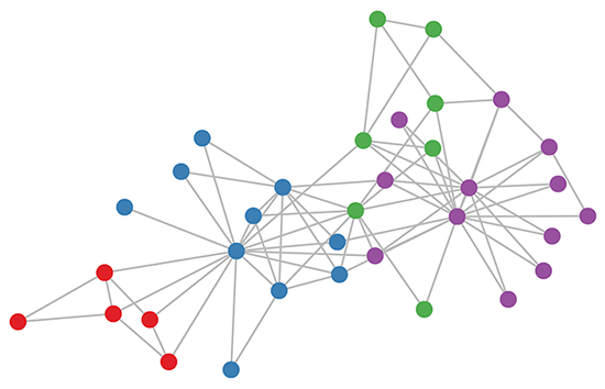
\[G=(V,E),\]where $V=\lbrace 1,\ldots,N\rbrace$ is a set of nodes and $E\subseteq V\times V$ is a set of edges. An edge $(j,i)$ will be written $j\rightarrow i$: node $j$ is its source and node $i$ its destination. An undirected relation $\lbrace i,j\rbrace$ is represented computationally by the two directed edges $i\rightarrow j$ and $j\rightarrow i$.
The combinatorial structure is usually accompanied by numerical attributes:
- a node-feature matrix $X\in\mathbb{R}^{N\times F}$, whose $i$-th row is $x_i$;
- optional edge attributes $e_{ji}\in\mathbb{R}^{F_e}$;
- targets defined at node, edge, or graph level.
For a molecular graph, nodes may denote atoms, edges may denote chemical bonds or spatial neighborhoods, and $x_i$ may encode atomic species and local descriptors. In a citation graph, nodes are documents, edges are citations, and node features may be derived from text.
1.2 Adjacency matrices and sparse edge lists
Fix the convention $A_{ij}=1$ when $j\rightarrow i$. The adjacency matrix $A\in\lbrace 0,1\rbrace^{N\times N}$ then encodes the graph, and the product $AX$ sums source-node features at their destinations. Although this notation is convenient for derivations, storing $A$ requires $O(N^2)$ memory.
Most graphs of practical interest are sparse: $\lvert E\rvert\ll N^2$. A coordinate representation therefore stores two integer arrays,
\[\mathbf{s}=(s_1,\ldots,s_{\lvert E\rvert}), \qquad \mathbf{d}=(d_1,\ldots,d_{\lvert E\rvert}),\]with $s_r\rightarrow d_r$ for edge $r$. In code, they are the tensors src and dst:
import torch

# Directed edges: 0→1, 1→0, 2→0, 2→3, 3→2
src = torch.tensor([0, 1, 2, 2, 3])
dst = torch.tensor([1, 0, 0, 3, 2])

x = torch.tensor([
    [1.0, 0.0],
    [0.8, 0.2],
    [0.0, 1.0],
    [0.1, 0.9],
])

# Gather one source representation per edge: shape [|E|, F].
x_source = x[src]
The expression x[src] is a gather operation: it moves data from node space to edge space. The reverse operation reduces edge messages at their destinations.
1.3 Learning problems on graphs
Graph prediction tasks differ in the object to which the target is attached.
| Task level | Input-output example | Typical final operation |
|---|---|---|
| Node | Assign a function or class to each atom | One prediction per node embedding |
| Edge | Predict whether two entities interact | Combine the two endpoint embeddings |
| Graph | Predict a molecular energy or material property | Pool all node embeddings, then regress |
The same message-passing backbone can serve all three settings. What changes is the prediction head and, for graph-level tasks, the readout that maps a variable number of nodes to a fixed-dimensional vector.
1.4 The absence of a canonical node order
Node indices are bookkeeping devices, not spatial coordinates. If a permutation matrix $P$ relabels the nodes, then
\[X' = PX, \qquad A' = PAP^\top\]describe the same attributed graph. A node-level graph network $f$ should be permutation equivariant:
\[f(PX,PAP^\top)=P f(X,A).\]A graph-level predictor should be invariant to the same relabeling. Parameter sharing across nodes and symmetric neighborhood reductions—sum, mean, or maximum—provide these properties. Concatenating neighbors in an arbitrary stored order would not.
2. Message passing as local computation
Let $h_i^{(0)}=x_i$. A message-passing layer at depth $\ell$ can be separated into three maps [1]. For every edge $j\rightarrow i$, a message is constructed:
\[m_{j\rightarrow i}^{(\ell)} = M^{(\ell)}\!\left( h_i^{(\ell)},h_j^{(\ell)},e_{ji} \right). \tag{1}\]Messages entering node $i$ are reduced by a permutation-invariant operator:
\[\bar m_i^{(\ell)} = \underset{j\in\mathcal N(i)}{\operatorname{AGG}} m_{j\rightarrow i}^{(\ell)}. \tag{2}\]Finally, the node state is updated:
\[h_i^{(\ell+1)} = U^{(\ell)}\!\left(h_i^{(\ell)},\bar m_i^{(\ell)}\right). \tag{3}\]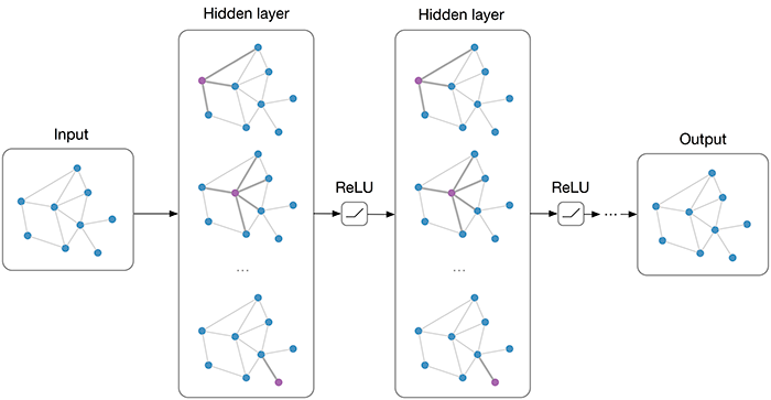
Equations (1)–(3) translate directly into PyTorch. For sum aggregation:
def message_passing(x, src, dst, message_fn, update_fn, edge_attr=None):
    source_x = x[src]
    destination_x = x[dst]

    if edge_attr is None:
        messages = message_fn(source_x, destination_x)
    else:
        messages = message_fn(source_x, destination_x, edge_attr)

    aggregated = messages.new_zeros(x.size(0), messages.size(-1))
    aggregated.index_add_(0, dst, messages)

    return update_fn(x, aggregated)
index_add_ is the essential sparse reduction: rows of messages sharing the same destination index are summed. Replacing it with a mean or elementwise maximum changes the aggregator but not the computational pattern.
After one layer, $h_i^{(1)}$ depends on the one-hop neighborhood of $i$. After $L$ layers, information can travel along paths of at most $L$ edges. Depth therefore controls the receptive field, but it also repeatedly mixes node states; this becomes relevant when oversmoothing is considered later.
3. Graph Convolutional Networks
3.1 Renormalized graph propagation
Kipf and Welling derive GCN as a first-order approximation to localized spectral graph convolution [2]. The resulting layer has a particularly simple spatial interpretation. First add one self-loop per node:
\[\widetilde A=A+I_N. \tag{4}\]The self-loop retains direct access to the node’s current representation during aggregation. Define the corresponding degree matrix
\[\widetilde D_{ii}=\sum_j \widetilde A_{ij}, \tag{5}\]and the symmetrically normalized propagation operator
\[\widehat A=\widetilde D^{-1/2}\widetilde A\widetilde D^{-1/2}. \tag{6}\]A GCN layer is then
\[H^{(\ell+1)}=\sigma\!\left( \widehat A H^{(\ell)}W^{(\ell)}+b^{(\ell)} \right). \tag{7}\]Here $W^{(\ell)}\in\mathbb{R}^{F_\ell\times F_{\ell+1}}$ is learned, while $\widehat A$ is determined by graph structure. Equation (7) can be read at one destination node:
\[h_i^{(\ell+1)}=\sigma\!\left( \sum_{j\in\mathcal N(i)\cup\{i\}} \frac{1}{\sqrt{\widetilde d_i\widetilde d_j}} h_j^{(\ell)}W^{(\ell)}+b^{(\ell)} \right). \tag{8}\]Thus GCN is a message-passing layer with
\[m_{j\rightarrow i}^{(\ell)}= \frac{1}{\sqrt{\widetilde d_i\widetilde d_j}} h_j^{(\ell)}W^{(\ell)},\]sum aggregation, and a nonlinear update. The coefficient reduces the disproportionate influence of high-degree nodes. For an undirected graph, which is the setting assumed here, every edge is stored in both directions and the source and destination degrees are consistent with (6).
3.2 From the matrix equation to edge-index code
The normalization in (4)–(6) can be computed without materializing an $N\times N$ matrix:
def gcn_normalize(src, dst, num_nodes):
    nodes = torch.arange(num_nodes, device=src.device)

    # Equation (4): append i→i for every node i.
    src_hat = torch.cat([src, nodes])
    dst_hat = torch.cat([dst, nodes])

    # Equation (5): in-degree after adding self-loops.
    degree = torch.zeros(num_nodes, device=src.device)
    degree.index_add_(
        0,
        dst_hat,
        torch.ones_like(dst_hat, dtype=degree.dtype),
    )

    # One value of D^(-1/2) A D^(-1/2) per stored edge.
    norm = degree[src_hat].rsqrt() * degree[dst_hat].rsqrt()
    return src_hat, dst_hat, norm
The layer first transforms all nodes, gathers transformed source states, weights them, and finally scatter-sums them at destinations:
def gcn_layer(x, src, dst, weight, bias=None, activation=None):
    src_hat, dst_hat, norm = gcn_normalize(src, dst, x.size(0))

    transformed = x @ weight
    messages = norm.unsqueeze(-1) * transformed[src_hat]

    out = transformed.new_zeros(transformed.shape)
    out.index_add_(0, dst_hat, messages)

    if bias is not None:
        out = out + bias
    return activation(out) if activation is not None else out
The index_add_ statement is the sparse counterpart of left multiplication by $\widehat A$. Autograd records the gather, multiplication, and reduction operations, so loss.backward() differentiates the layer without a graph-specific library.
3.3 Interpretation and computational cost
GCN uses the same structural weighting rule for every sample and every feature channel. Its learnable component is the feature transformation $W^{(\ell)}$; its neighborhood coefficients depend only on degrees. With $F_\ell$ input and $F_{\ell+1}$ output channels, a sparse layer requires approximately
\[O\!\left(NF_\ell F_{\ell+1}+|E|F_{\ell+1}\right)\]operations: one dense node-wise transform and one sparse propagation. This simplicity makes GCN a strong baseline, particularly on homophilous graphs where adjacent nodes tend to share labels or signals.
Its restriction is equally clear. Two neighbors with the same degrees receive the same scalar structural coefficient, regardless of their current features or relevance to the prediction.
4. Graph Attention Networks
4.1 Feature-dependent neighborhood weights
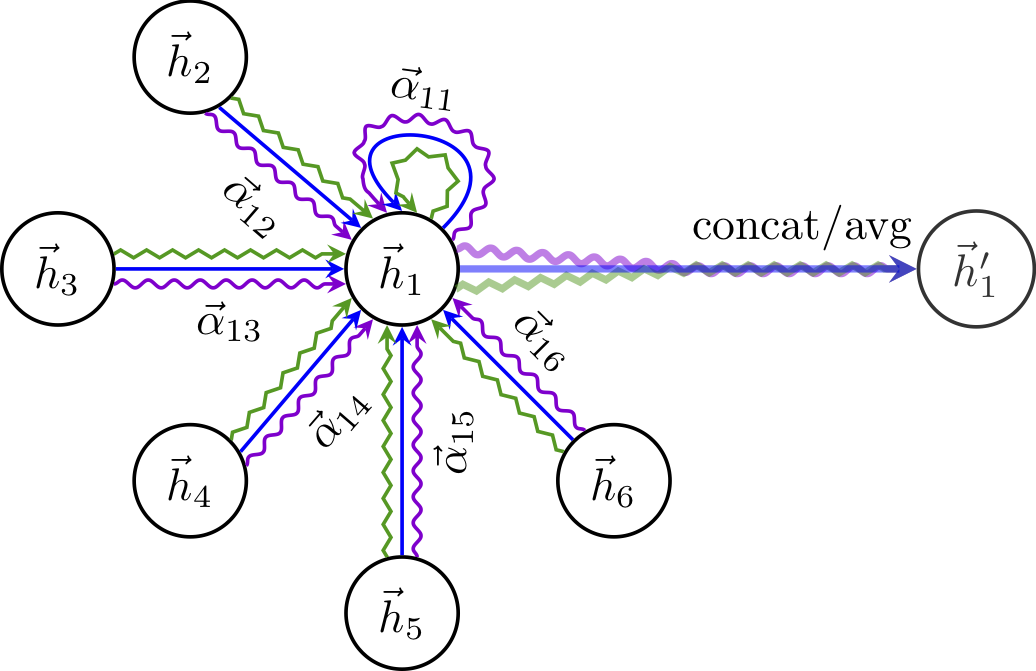
GAT retains local aggregation but learns the coefficient assigned to each edge [3]. For one attention head, transform each node:
\[z_i=Wh_i, \qquad W\in\mathbb{R}^{F\times F'}. \tag{9}\]For an edge $j\rightarrow i$, the original GAT score is
\[e_{ji}=\operatorname{LeakyReLU}\!\left( a^\top[z_j\,\Vert\,z_i] \right), \tag{10}\]where $a\in\mathbb{R}^{2F’}$ is learned and $\Vert$ denotes concatenation. Partitioning $a=[a_{\mathrm{src}}\Vert a_{\mathrm{dst}}]$ avoids explicitly constructing the concatenated tensor:
\[e_{ji}=\operatorname{LeakyReLU}\!\left( a_{\mathrm{src}}^\top z_j+a_{\mathrm{dst}}^\top z_i \right). \tag{11}\]import torch.nn.functional as F
def gat_logits(x, src, dst, weight, attn_src, attn_dst):
z = x @ weight # Equation (9)
logits = (
(z[src] * attn_src).sum(dim=-1)
+ (z[dst] * attn_dst).sum(dim=-1)
)
return F.leaky_relu(logits, negative_slope=0.2), z
The score is meaningful only relative to other edges entering the same node. A neighborhood-wise softmax gives
\[\alpha_{ji}= \frac{\exp(e_{ji})} {\sum_{k\in\mathcal N(i)\cup\{i\}}\exp(e_{ki})}, \qquad \sum_{j\in\mathcal N(i)\cup\{i\}}\alpha_{ji}=1. \tag{12}\]The grouping by destination is essential. A single softmax over all graph edges would couple unrelated neighborhoods and would not implement (12).
def neighborhood_softmax(logits, dst, num_nodes):
    alpha = torch.zeros_like(logits)

    # Deliberately explicit; optimized implementations use segment kernels.
    for node in range(num_nodes):
        incoming = dst == node
        if incoming.any():
            alpha[incoming] = torch.softmax(logits[incoming], dim=0)

    return alpha
The destination receives the attention-weighted sum
\[h_i'=\sigma\!\left( \sum_{j\in\mathcal N(i)\cup\{i\}} \alpha_{ji}z_j \right). \tag{13}\]def gat_head(x, src, dst, weight, attn_src, attn_dst,
bias=None, activation=None):
# GAT normally attends to the node itself as well.
nodes = torch.arange(x.size(0), device=x.device)
src_hat = torch.cat([src, nodes])
dst_hat = torch.cat([dst, nodes])
logits, z = gat_logits(
x, src_hat, dst_hat, weight, attn_src, attn_dst
)
alpha = neighborhood_softmax(logits, dst_hat, x.size(0))
messages = alpha.unsqueeze(-1) * z[src_hat]
out = z.new_zeros(z.shape)
out.index_add_(0, dst_hat, messages)
if bias is not None:
out = out + bias
if activation is not None:
out = activation(out)
return out, alpha
4.2 Multiple attention heads
GAT stabilizes learning by using $K$ independently parameterized heads. Hidden layers usually concatenate their outputs,
\[h_i'=\mathbin\Vert_{k=1}^{K} \sigma\!\left( \sum_{j\in\mathcal N(i)\cup\{i\}} \alpha_{ji}^{(k)}W^{(k)}h_j \right), \tag{14}\]whereas a final layer may average them:
\[h_i'=\frac{1}{K}\sum_{k=1}^{K} \sum_{j\in\mathcal N(i)\cup\{i\}} \alpha_{ji}^{(k)}W^{(k)}h_j. \tag{15}\]In PyTorch, the merge itself is elementary:
hidden = torch.cat(head_outputs, dim=-1)           # Equation (14)
prediction = torch.stack(head_outputs).mean(dim=0) # Equation (15)
Each head adds its own node transform and edge scores. The approximate sparse cost is
\[O\!\left( K\left[NFF'+\lvert E\rvert F'\right] \right),\]and $K\lvert E\rvert$ attention values must be represented during the forward pass. GAT is consequently more flexible than GCN, but not free.
4.3 What attention does—and does not—provide
The coefficients $\alpha_{ji}$ are conditional on learned representations and can reveal which neighbors receive large weights in a particular layer. They are not, by themselves, a causal or faithful explanation of the final prediction. Later transformations, nonlinearities, redundant features, and interactions between heads can all alter their interpretation. Attention should therefore be inspected as an internal routing quantity, not treated automatically as an explanation [5].
5. From node representations to predictions
For semi-supervised node classification, a final graph layer returns logits $o_i\in\mathbb{R}^{C}$. Cross-entropy is evaluated only on labeled training nodes $V_{\mathrm{train}}$:
\[\mathcal L_{\mathrm{node}}= -\frac{1}{|V_{\mathrm{train}}|} \sum_{i\in V_{\mathrm{train}}} \log\frac{\exp(o_{i,y_i})}{\sum_{c=1}^{C}\exp(o_{i,c})}. \tag{16}\]For graph regression, node states must first be pooled. A mean readout for graph $G_b$ is
\[g_b=\frac{1}{|V_b|}\sum_{i\in V_b}h_i^{(L)}, \qquad \widehat y_b=w^\top g_b+c. \tag{17}\]def global_mean_pool(node_embeddings, batch, num_graphs):
pooled = node_embeddings.new_zeros(num_graphs, node_embeddings.size(-1))
pooled.index_add_(0, batch, node_embeddings)
count = node_embeddings.new_zeros(num_graphs)
count.index_add_(0, batch, torch.ones_like(batch, dtype=count.dtype))
return pooled / count.clamp_min(1).unsqueeze(-1)
The pooling operation must be permutation invariant. Sum, mean, and maximum are common choices, but they encode different assumptions about graph size and multiplicity.
6. Controlled GCN–GAT comparison
The companion code includes a small benchmark intended to expose model behavior, not to establish a general ranking. All data are synthetic; every value below is a mean $\pm$ sample standard deviation over seeds $0,1,2$.
6.1 Experimental protocol
| Component | Protocol |
|---|---|
| Node classification | One 90-node, balanced three-class stochastic block model per seed; stratified 60%/20%/20% split |
| Homophily regimes | High: $p_{\mathrm{in}}=0.35$, $p_{\mathrm{out}}=0.02$; moderate: $0.25/0.08$; low: $0.18/0.12$ |
| Graph regression | 72 graphs per seed, each with 8–14 nodes; 70%/15%/remainder split |
| Capacity | Two message-passing layers, hidden width 16; one attention head for GAT |
| Training | Adam, validation-loss early stopping, identical data splits and stopping rules |
| Deep-model diagnostic | Separate six-layer classifiers in the moderate-homophily regime |
Holding width and depth fixed does not make the parameter counts identical: attention introduces additional vectors. The node classifiers contain 467 parameters for GCN and 531 for GAT.
6.2 Node classification
| Homophily | Model | Test accuracy $\uparrow$ | Macro-F1 $\uparrow$ |
|---|---|---|---|
| High | GCN | $0.981\pm0.032$ | $0.981\pm0.032$ |
| High | GAT | $1.000\pm0.000$ | $1.000\pm0.000$ |
| Moderate | GCN | $0.593\pm0.179$ | $0.576\pm0.181$ |
| Moderate | GAT | $0.574\pm0.085$ | $0.542\pm0.108$ |
| Low | GCN | $0.333\pm0.111$ | $0.269\pm0.062$ |
| Low | GAT | $0.315\pm0.085$ | $0.243\pm0.105$ |
Both architectures solve the high-homophily setting, where adjacency is strongly aligned with class membership. As $p_{\mathrm{in}}-p_{\mathrm{out}}$ narrows, the graph becomes less informative and performance approaches the balanced three-class chance accuracy of $1/3$.
The moderate- and low-homophily means favor GCN slightly, but the uncertainty across three seeds is large. These results do not support the claim that one architecture is generally superior. They show instead that learnable attention cannot recover class information that is largely absent from both features and local connectivity.
6.3 Graph regression
The graph target combines node features and degree statistics. Targets are standardized using training-set statistics and transformed back to their original scale for evaluation.
| Model | Test MAE $\downarrow$ | Test RMSE $\downarrow$ | Test $R^2$ $\uparrow$ |
|---|---|---|---|
| GCN | $0.162\pm0.025$ | $0.214\pm0.017$ | $0.250\pm0.365$ |
| GAT | $0.171\pm0.074$ | $0.215\pm0.097$ | $0.114\pm0.713$ |
The mean absolute and root-mean-square errors are close relative to their variation. The unstable $R^2$ values reflect a small synthetic test set. A larger study would require more graphs, more seeds, capacity-matched variants, and confidence intervals chosen before interpreting model differences.
6.4 Oversmoothing
Repeated neighborhood averaging can make node representations increasingly similar. Two complementary statistics are recorded after every layer. Mean off-diagonal cosine similarity is
\[S^{(\ell)}= \frac{1}{N(N-1)} \sum_{i\ne j} \frac{\left(h_i^{(\ell)}\right)^\top h_j^{(\ell)}} {\|h_i^{(\ell)}\|_2\,\|h_j^{(\ell)}\|_2}, \tag{18}\]and normalized dispersion is
\[D^{(\ell)}= \frac{\sum_i\|h_i^{(\ell)}-\bar h^{(\ell)}\|_2^2} {\sum_i\|h_i^{(\ell)}\|_2^2+\varepsilon}. \tag{19}\]Larger $S^{(\ell)}$ and smaller $D^{(\ell)}$ indicate more aligned representations.
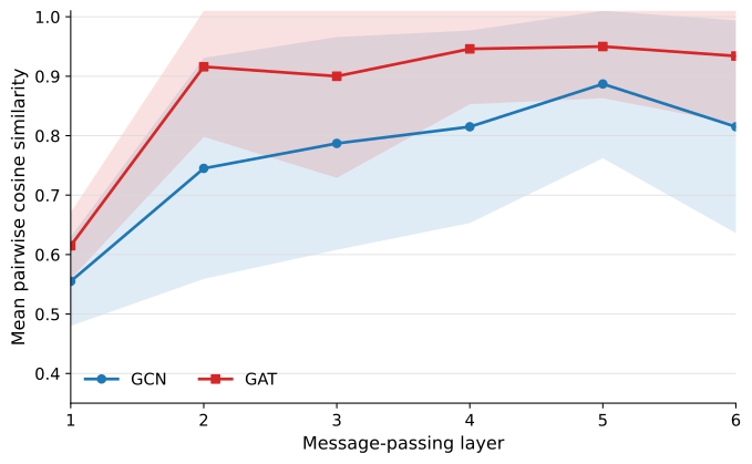
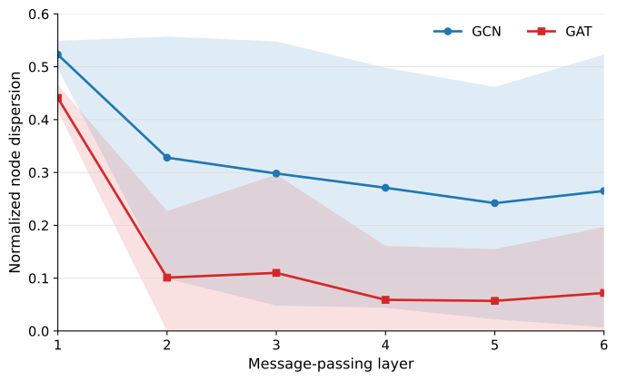
| Layer | GCN cosine $\uparrow$ | GAT cosine $\uparrow$ | GCN dispersion $\downarrow$ | GAT dispersion $\downarrow$ |
|---|---|---|---|---|
| 1 | $0.555\pm0.075$ | $0.615\pm0.056$ | $0.523\pm0.026$ | $0.441\pm0.025$ |
| 2 | $0.745\pm0.186$ | $0.916\pm0.118$ | $0.328\pm0.229$ | $0.101\pm0.126$ |
| 3 | $0.787\pm0.179$ | $0.900\pm0.171$ | $0.298\pm0.250$ | $0.110\pm0.186$ |
| 4 | $0.815\pm0.162$ | $0.946\pm0.093$ | $0.271\pm0.227$ | $0.059\pm0.102$ |
| 5 | $0.887\pm0.125$ | $0.950\pm0.087$ | $0.242\pm0.220$ | $0.057\pm0.098$ |
| 6 | $0.815\pm0.179$ | $0.934\pm0.114$ | $0.265\pm0.258$ | $0.072\pm0.125$ |
At layer six, test accuracy is $0.593\pm0.280$ for GCN and $0.481\pm0.257$ for GAT. Attention has not prevented representation alignment in this configuration. This is not a universal statement about GAT: it is an observation for one synthetic distribution, one head, one width, and one optimization protocol. Its value is methodological—oversmoothing should be measured rather than inferred from the architecture’s name.
7. Structural comparison
| Property | GCN | GAT |
|---|---|---|
| Edge coefficient | $1/\sqrt{\widetilde d_i\widetilde d_j}$ | $\alpha_{ji}$ from endpoint states |
| Learned quantities | Feature transform $W$ | $W$ and attention vector $a$ per head |
| Neighborhood normalization | Symmetric degree normalization | Destination-wise softmax |
| Data dependence | Coefficients fixed for a given graph | Coefficients change with node states |
| Sparse memory | $O(\lvert E\rvert)$ coefficients | $O(K\lvert E\rvert)$ attention coefficients |
| Principal strength | Simplicity and parameter efficiency | Adaptive neighbor weighting |
| Principal limitation | Same structural rule for all examples | Additional parameters and edge-wise computation |
The models share more than this table may suggest. Both are local, permutation-equivariant message-passing networks. Both require a deliberate self-loop convention. Both depend on the information present in the chosen neighborhood graph. Both can lose discriminative node information with depth. The choice between them is therefore empirical and should be made under a controlled protocol rather than from the expectation that attention must improve every task.
8. Reproducibility and implementation map
The full repository separates the implementation into graph primitives, generic message passing, graph convolution, graph attention, readout, datasets, optimization, and experiments. It contains:
- sparse COO graph construction and gather/scatter reductions;
- GCN normalization and propagation;
- single- and multi-head GAT operations;
- node-classification and graph-regression pipelines;
- raw multi-seed benchmark results and oversmoothing diagnostics.
git clone https://github.com/rizkisalaheddine/message-passing-gnns-from-scratch.git
cd message-passing-gnns-from-scratch
python -m venv .venv
source .venv/bin/activate
python -m pip install -r requirements.txt
python demo.py
To reproduce the comparison tables:
python -m gnn_from_scratch.experiments.benchmark \
  --output results/gcn_gat_benchmark.json
The code favors inspectability over optimized segment kernels. Its CPU timings should not be compared with PyTorch Geometric or other production libraries; the purpose is to expose the computation that those libraries implement efficiently.
9. Conclusion
Message passing provides a compact language for neural computation on graphs: construct an edge-wise message, reduce messages at destinations, and update node states. GCN instantiates this scheme with fixed symmetric degree normalization. GAT replaces the fixed coefficient with a learned neighborhood softmax, usually replicated across several heads.
Writing both layers with src, dst, gather operations, and index_add_ makes their relationship explicit. The apparent difference between graph convolution and graph attention is not a difference in computational substrate; it is primarily a choice of how local messages are weighted. That observation is the useful starting point for more elaborate models involving edge features, geometric equivariance, heterogeneous relations, or learned molecular interactions.
References
- J. Gilmer, S. S. Schoenholz, P. F. Riley, O. Vinyals, and G. E. Dahl, “Neural Message Passing for Quantum Chemistry,” Proceedings of ICML, 2017.
- T. N. Kipf and M. Welling, “Semi-Supervised Classification with Graph Convolutional Networks,” Proceedings of ICLR, 2017.
- P. Veličković et al., “Graph Attention Networks,” Proceedings of ICLR, 2018.
- K. Oono and T. Suzuki, “Graph Neural Networks Exponentially Lose Expressive Power for Node Classification,” Proceedings of ICLR, 2020.
- S. Jain and B. C. Wallace, “Attention is not Explanation,” Proceedings of NAACL-HLT, 2019.
Pedagogical sources
- F. Karami, “Understanding Graph Attention Networks: A Practical Exploration,” 2023.
- M. Labonne, “Graph Convolutional Networks: Introduction to GNNs,” 2023.